MPT Part 1: Two Securities Portfolio
Published:
Modelling and visualisation on some of the financial engineering theorems using Jupyter Notebook. The mathematics of the theorems follow the book: Capinski, M. and Zastawniak, T. (2011). Mathematics for Finance. An Introduction to Financial Engineering (Second Edition).
Check the Jupyter Notebook in my Github repository Python-for-mathematical-finance , or run the code in Google Colab MPT Part 1 - Two Securities Portfolio .
Table of Contents
Two Securities Portfolio
import numpy as np
import matplotlib as mpl
import matplotlib.pyplot as plt
import matplotlib.colors as mcolors
import matplotlib.patches as mpatches
import scipy.stats as stats
import pandas as pd
import pandas_datareader as pdr
import random
from adjustText import adjust_text
from tqdm.notebook import tqdm
tqdm.pandas()
Theorems for the feasible set
For two risky assets, the portfolio return is:
\[\begin{equation} \mu_{v} = w_1 \mu_1 + w_2 \mu_2, \end{equation}\]and the variance is:
\[\begin{equation} \sigma^2_V = w^2_1 \sigma^2_1 + w^2_2 \sigma^2_2 + 2w_1w_2c_{12}. \end{equation}\]Here, $w_1, w_2 \in \mathbb{R}$, and $1 = w_1 + w_2$.
We use $s$ to represent the $w_1$, then the $w_2 = 1 - s$. The above equation would be:
\[\begin{equation*} \mu_{v} = s \mu_1 + (1-s) \mu_2, \end{equation*}\] \[\begin{equation*} \sigma^2_V = s^2 \sigma^2_1 + (1-s)^2 \sigma^2_2 + 2s(1-s)c_{12}. \end{equation*}\]Here $s \in \mathbb{R}$.
If $\rho < 1$, or $\sigma_1 \neq \sigma_2$, the weight of asset 1, $s_0$, with mimimum varaince $\sigma_V^2$, will be:
\[\begin{equation} s_0 = \frac{\sigma_2^2 - c_{12}}{\sigma_1^2+\sigma_2^2-2c_{12}}, \end{equation}\]And the expected return $\mu_V$ and variance $\sigma_V^2$ will be:
\[\begin{equation} \mu_0=\frac{\mu_1\sigma_2^2+\mu_2\sigma_1^2-(\mu_1+\mu_2)c_{12}}{\sigma_1^2+\sigma_2^2-2c_{12}}, \end{equation}\] \[\begin{equation} \sigma_0^2=\frac{\sigma_1^2\sigma_2^2-c_{12}^2}{\sigma_1^2+\sigma_2^2-2c_{12}}. \end{equation}\]If $-1<\rho_{12}<1$ and $\mu_1\neq mu_2$, then for each feasible set in the portfolio $V$, $x=\sigma_V$ and $y=\mu_V$ satisfy the following equation:
\[\begin{equation} x^2-A^2(y-\mu_0)^2=\sigma_0^2, \end{equation}\]where
\[\begin{equation*} A^2 = \frac{\sigma_1^2+\sigma_2^2-2c_{12}}{(\mu_1-\mu_2)^2}>0, \end{equation*}\]whose asymptotes are:
\[\begin{equation*} y=\mu_0 \pm \frac{1}{A}x. \end{equation*}\]# When separate_plot=True (default), the corr12 should be a digit imput.
# When separate_plot=False, the corr12 needs to be a list of situations.
def two_asset_plot(mu1, mu2, var1, var2, corr12, separate_plot=True):
def strategy_idfier(weight):
strat_ls = ["long", "short", "ignore"]
if weight>0:
strategy = strat_ls[0]
elif weight<0:
strategy = strat_ls[1]
else:
strategy = strat_ls[2]
return strategy
if separate_plot:
if var2 == 0:
var_rf = var2
var2 += 0.0000000000001
else:
var_rf = var2
cov12 = corr12*np.sqrt(var1)*np.sqrt(var2)
s0 = (var2-cov12)/(var1+var2-2*cov12)
mu0 = (mu1*var2+mu2*var1-(mu1+mu2)*cov12)/(var1+var2-2*cov12)
var0 = (var1*var2-cov12**2)/(var1+var2-2*cov12)
sd1sd2 = np.sqrt(var1)/np.sqrt(var2)
if var_rf == 0:
print("[Special situation]: one risky, another risk free")
else:
if corr12 == 1:
print("[Situation 1]: correlation equals 1")
elif corr12 > np.sqrt(var1)/np.sqrt(var2) and corr12 < 1:
print("[Situation 2]: correlation between STD1/STD2 (%s) and 1" %round(sd1sd2,4))
elif corr12 == np.sqrt(var1)/np.sqrt(var2):
print("[Situation 3]: correlation equals STD1/STD2 (%s)" %round(sd1sd2,4))
elif corr12 < np.sqrt(var1)/np.sqrt(var2) and corr12 > -1:
print("[Situation 4]: correlation between -1 and STD1/STD2 (%s)" %round(sd1sd2,4))
elif corr12 == -1:
print("[Situation 5]: correlation equals -1")
else:
print("[Error: correlation out of range]")
print("MVP strategy (weight): %s asset 1 (%s%%), and %s asset 2 (%s%%)"
%(strategy_idfier(round(s0,4)),round(100*s0,2),strategy_idfier(round(1-s0,4)),round(100*(1-s0),2)))
print("Return of MVP: %s" % round(mu0,4))
print("Minimum variance: %s" % round(var0,4))
print("Covariance: %s" % round(cov12,4))
f = plt.figure(figsize = (10,8))
ax = f.add_subplot(1, 1, 1)
x = np.linspace(0, max((np.sqrt(var1),np.sqrt(var2)))*(5/3), 400)
y = np.linspace(min(mu1,mu2,mu0)-np.abs(2/3)*max(mu1,mu2,mu0), max(mu1,mu2,mu0)+np.abs((2/3)*max(mu1,mu2,mu0)), 400)
x, y = np.meshgrid(x, y)
x2 = np.linspace(0, max(np.sqrt(var1),np.sqrt(var2),np.sqrt(np.abs(var0)))*(5/3))
y2 = mu0+np.sqrt((((mu1-mu2)**2)/(var1+var2-2*cov12)))*x2
y3 = mu0-np.sqrt((((mu1-mu2)**2)/(var1+var2-2*cov12)))*x2
plt.plot(x2, y2,color='grey',lw=1,ls='--')
plt.plot(x2, y3,color='grey',lw=1,ls='--')
formula = ((y-mu0)**2-(x**2-var0)*(((mu1-mu2)**2)/(var1+var2-2*cov12)))
masked_long = (y<min(mu1,mu2))|(max(mu1,mu2)<y)
masked_short = (y>=min(mu1,mu2))&(y<=max(mu1,mu2))
plt.contour(np.ma.masked_where(masked_long,x),np.ma.masked_where(masked_long,y),np.ma.masked_where(masked_long,formula), [0], colors='deepskyblue', linestyles='-')
plt.contour(np.ma.masked_where(masked_short,x),np.ma.masked_where(masked_short,y),np.ma.masked_where(masked_short,formula), [0], colors='deepskyblue', linestyles='--')
plt.hlines(mu0,0,np.sqrt(np.abs(var0)),color='grey',lw=1,ls='--')
plt.vlines(np.sqrt(np.abs(var0)),0,mu0,color='grey',lw=1,ls='--')
two_assets = [[np.sqrt(var1), np.sqrt(var2)], [mu1, mu2]]
plt.scatter(*two_assets, marker='v', color='red')
text1 = plt.text(np.sqrt(var1), mu1, "(σ1, μ1)")
text2 = plt.text(np.sqrt(var2), mu2, "(σ2, μ2)")
min_var = [[np.sqrt(np.abs(var0))], [mu0]]
plt.scatter(*min_var, marker='x', color='purple')
text3 = plt.text(np.sqrt(np.abs(var0)), mu0, "Min(σ)")
adjust_text([text1, text2, text3])
plt.xlabel("Standard Deviation (σ)")
plt.ylabel("Expected Return (μ)")
ax.spines['left'].set_position('zero')
ax.spines['bottom'].set_position('zero')
ax.spines['right'].set_color('none')
ax.spines['top'].set_color('none')
ax.xaxis.set_ticks_position('bottom')
ax.yaxis.set_ticks_position('left')
plt.show()
else:
if var2 == 0:
var_rf = var2
var2 += 0.0000000000001
else:
var_rf = var2
sd1sd2 = np.sqrt(var1)/np.sqrt(var2)
print("STD1/STD2 = %s" %round(sd1sd2,4))
f = plt.figure(figsize = (10,10))
ax = f.add_subplot(1, 1, 1)
color_idx = 0
colorlabel = {}
for situation in corr12:
cov12 = situation*np.sqrt(var1)*np.sqrt(var2)
s0 = (var2-cov12)/(var1+var2-2*cov12)
mu0 = (mu1*var2+mu2*var1-(mu1+mu2)*cov12)/(var1+var2-2*cov12)
var0 = (var1*var2-cov12**2)/(var1+var2-2*cov12)
if var_rf == 0:
print("[Special situation]: one risky, another risk free")
else:
print("[Situation %s] MVP: (%s, %s), covariance = %s;" %(color_idx+1, round(np.sqrt(np.abs(var0)),4), round(mu0,4), round(cov12,4)))
print("MVP strategy (weight): %s asset 1 (%s%%), and %s asset 2 (%s%%)"
%(strategy_idfier(round(s0,4)),round(100*s0,2),strategy_idfier(round(1-s0,4)),round(100*(1-s0),2)))
x = np.linspace(0, max((np.sqrt(var1),np.sqrt(var2)))*(5/3), 400)
y = np.linspace(min(mu1,mu2,mu0)-np.abs(2/3)*max(mu1,mu2,mu0), max(mu1,mu2,mu0)+np.abs((2/3)*max(mu1,mu2,mu0)), 400)
x, y = np.meshgrid(x, y)
two_assets = [[np.sqrt(var1), np.sqrt(var2)], [mu1, mu2]]
plt.scatter(*two_assets, marker='v', color='red')
formula = ((y-mu0)**2-(x**2-var0)*(((mu1-mu2)**2)/(var1+var2-2*cov12)))
masked_long = (y<min(mu1,mu2))|(max(mu1,mu2)<y)
masked_short = (y>=min(mu1,mu2))&(y<=max(mu1,mu2))
color = list(mcolors.TABLEAU_COLORS.values())
plt.contour(np.ma.masked_where(masked_long,x),np.ma.masked_where(masked_long,y),np.ma.masked_where(masked_long,formula), [0], colors=color[color_idx], linestyles='-')
plt.contour(np.ma.masked_where(masked_short,x),np.ma.masked_where(masked_short,y),np.ma.masked_where(masked_short,formula), [0], colors=color[color_idx], linestyles='--')
colorlabel["Situation %s" %(color_idx+1)] = color[color_idx]
color_idx += 1
plt.hlines(mu0,0,np.sqrt(np.abs(var0)),color='grey',lw=1,ls='--')
plt.vlines(np.sqrt(np.abs(var0)),0,mu0,color='grey',lw=1,ls='--')
min_var = [[np.sqrt(np.abs(var0))], [mu0]]
plt.scatter(*min_var, marker='x', color='purple')
text1 = plt.text(np.sqrt(var1), mu1, "(σ1, μ1)")
text2 = plt.text(np.sqrt(var2), mu2, "(σ2, μ2)")
adjust_text([text1,text2])
fake_handles = [mpatches.Patch(color=item) for item in colorlabel.values()]
plt.legend(fake_handles, colorlabel.keys(), loc='upper left', prop={'size': 10})
plt.xlabel("Standard Deviation (σ)")
plt.ylabel("Expected Return (μ)")
ax.spines['left'].set_position('zero')
ax.spines['bottom'].set_position('zero')
ax.spines['right'].set_color('none')
ax.spines['top'].set_color('none')
ax.xaxis.set_ticks_position('bottom')
ax.yaxis.set_ticks_position('left')
plt.show()
Simulation with predefined returns and variances
First, we can manually simulate the expected return and the variance of two assets, and the correlation between two assets, and see what the plot will be.
Variables are:
mu1andmu2: $\mu_{1}$ and $\mu_{2}$, the expected return of asset 1 and 2.var1andvar2: $\sigma_{1}$ and $\sigma_{2}$, the variance of asset 1 and 2 ($\sigma_1 \neq \sigma_2$).corr12: $\rho_{12}$, the correlation between asset 1 and 2. $\rho_{12}=\frac{c_{12}}{\sigma_1\sigma_2}, \rho_{12} \in [-1,1]$
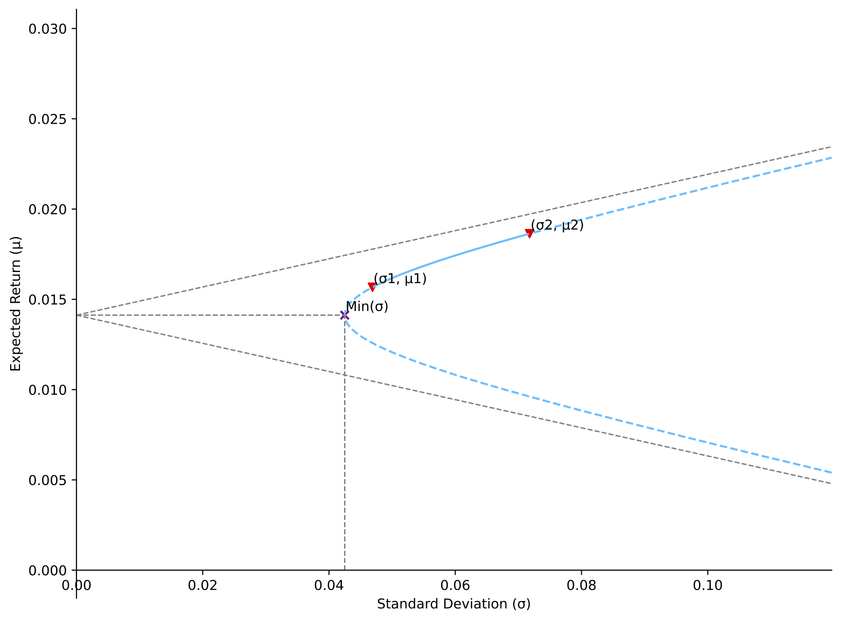
mu1 = 0.02
mu2 = 0.03
var1 = 0.015
var2 = 0.03
# corr12 = np.sqrt(var1)/np.sqrt(var2)
corr12 = random.uniform(-1,1)
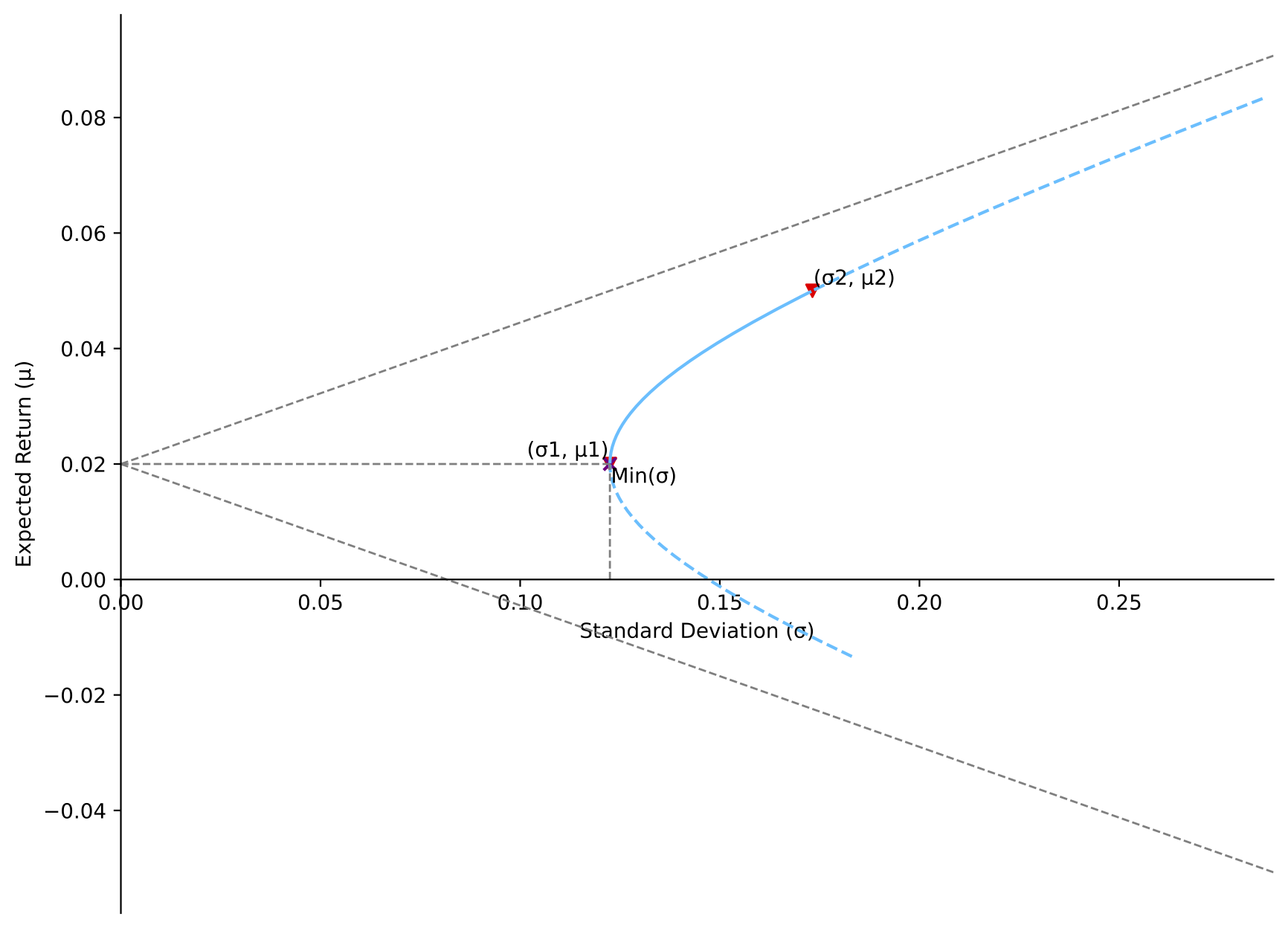
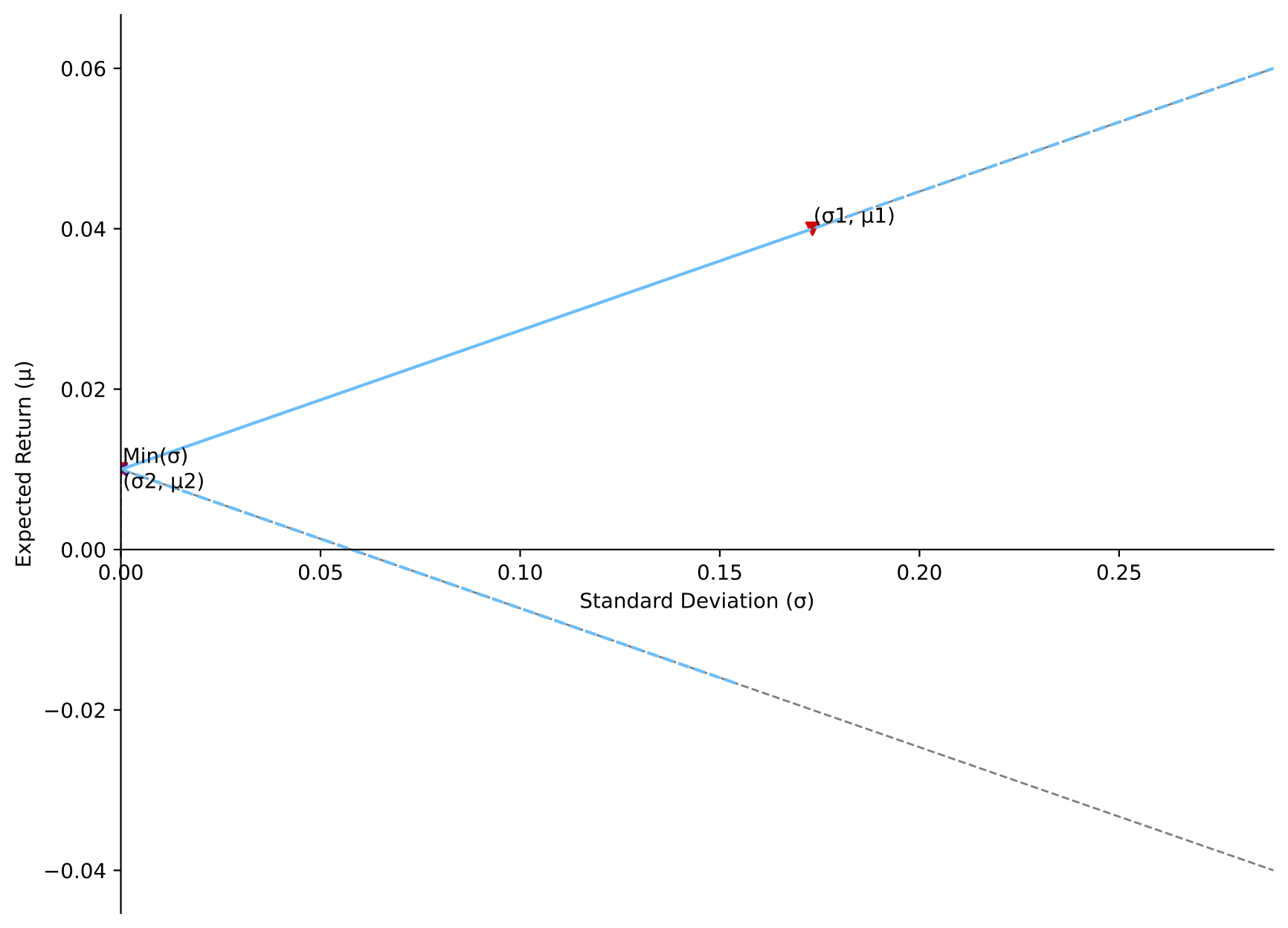
two_asset_plot(mu1, mu2, var1, var2, corr12)
[Situation 2]: correlation between STD1/STD2 (0.7071) and 1
MVP strategy (weight): long asset 1 (129.14%), and short asset 2 (-29.14%)
Return of MVP: 0.0171
Minimum variance: 0.0142
Covariance: 0.0178
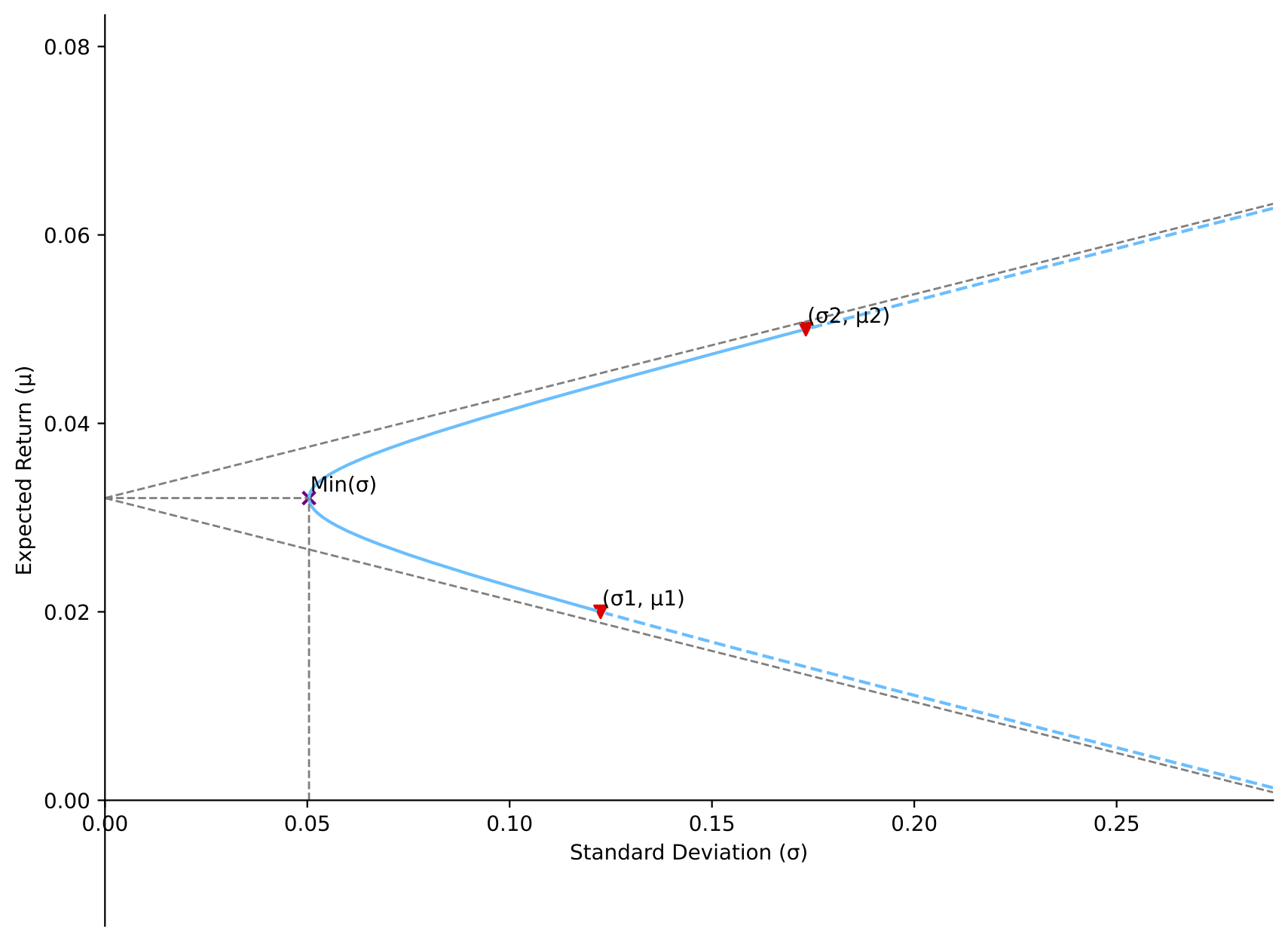
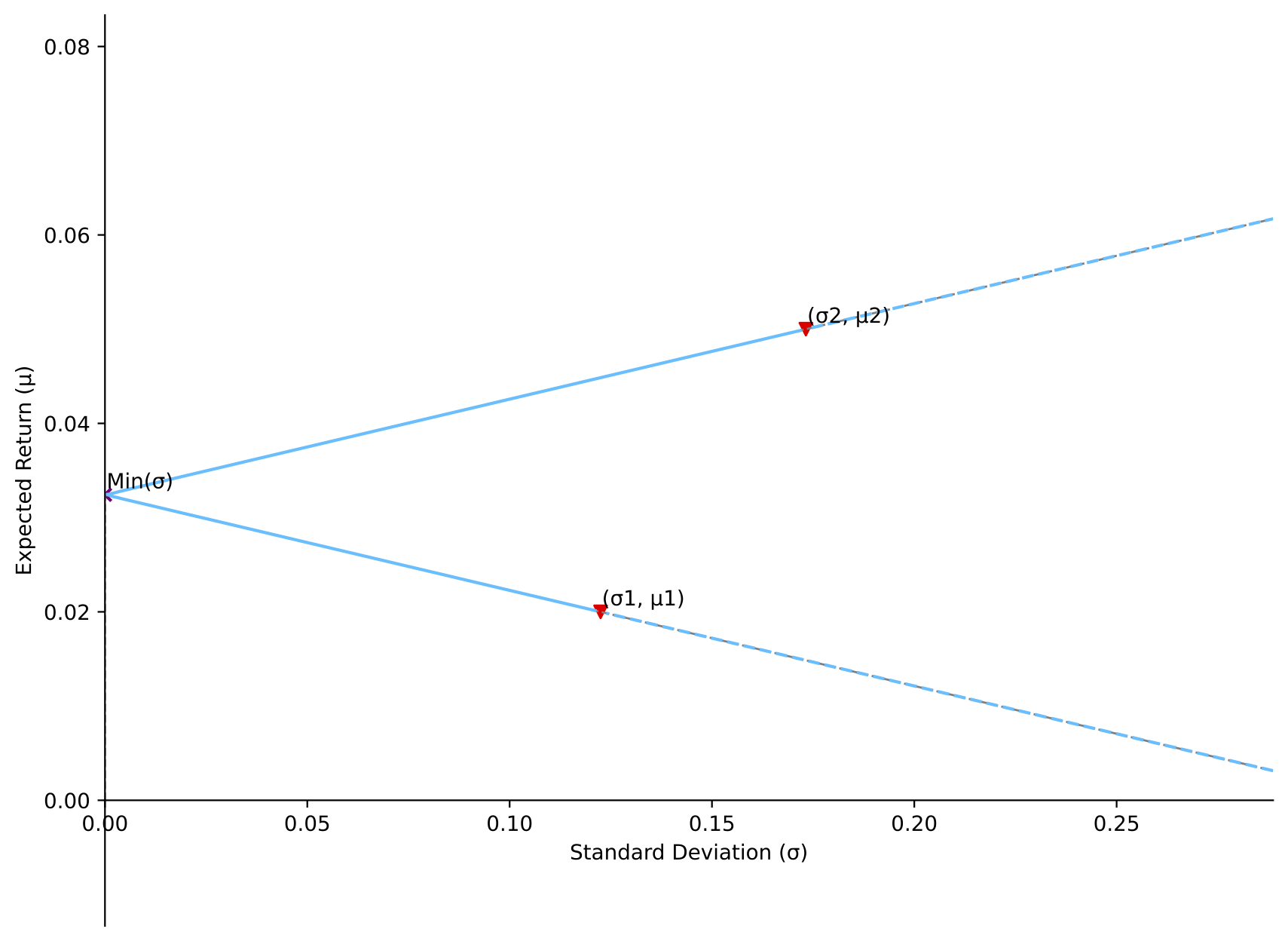
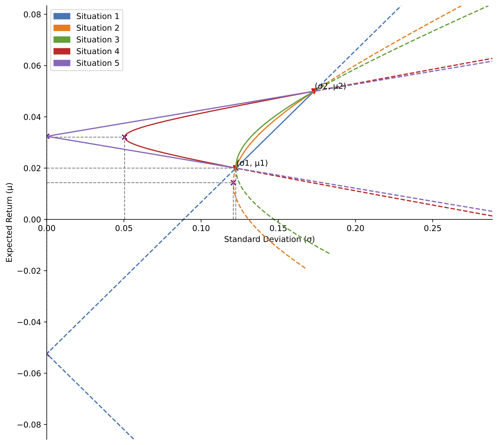
Assume $\sigma_1 \leq \sigma_2$, the plausible situations are:
If $\rho = 1$, there is a feasible set with short selling such that $\sigma_V=0$.
If $\frac{\sigma_1}{\sigma_2}<\rho<1$, the feasible set includes a short position, and $\sigma_V<\sigma_1$. But for every set without short selling, $\sigma_V\geq \sigma_1$.
If $\rho = \frac{\sigma_1}{\sigma_2}$, for every attainable set, $\sigma_V \geq \sigma_1$.
If $-1<\rho<\frac{\sigma_1}{\sigma_2}$, the feasible set without short selling has $\sigma_V<\sigma_1$.
If $\rho = -1$, a feasible set without short selling has $\sigma_V=0$.
# Separate plots for the five situations above
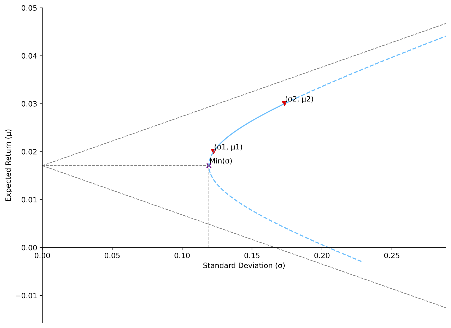
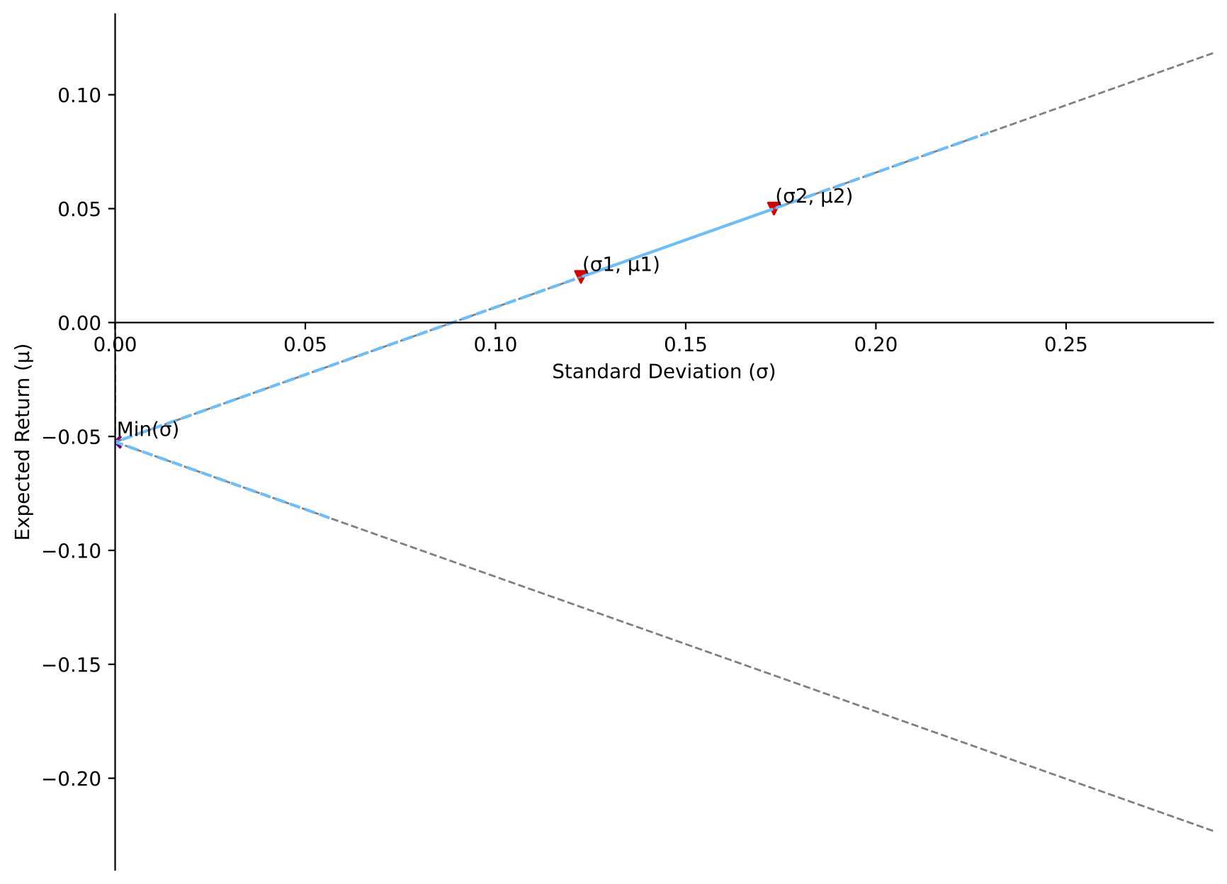
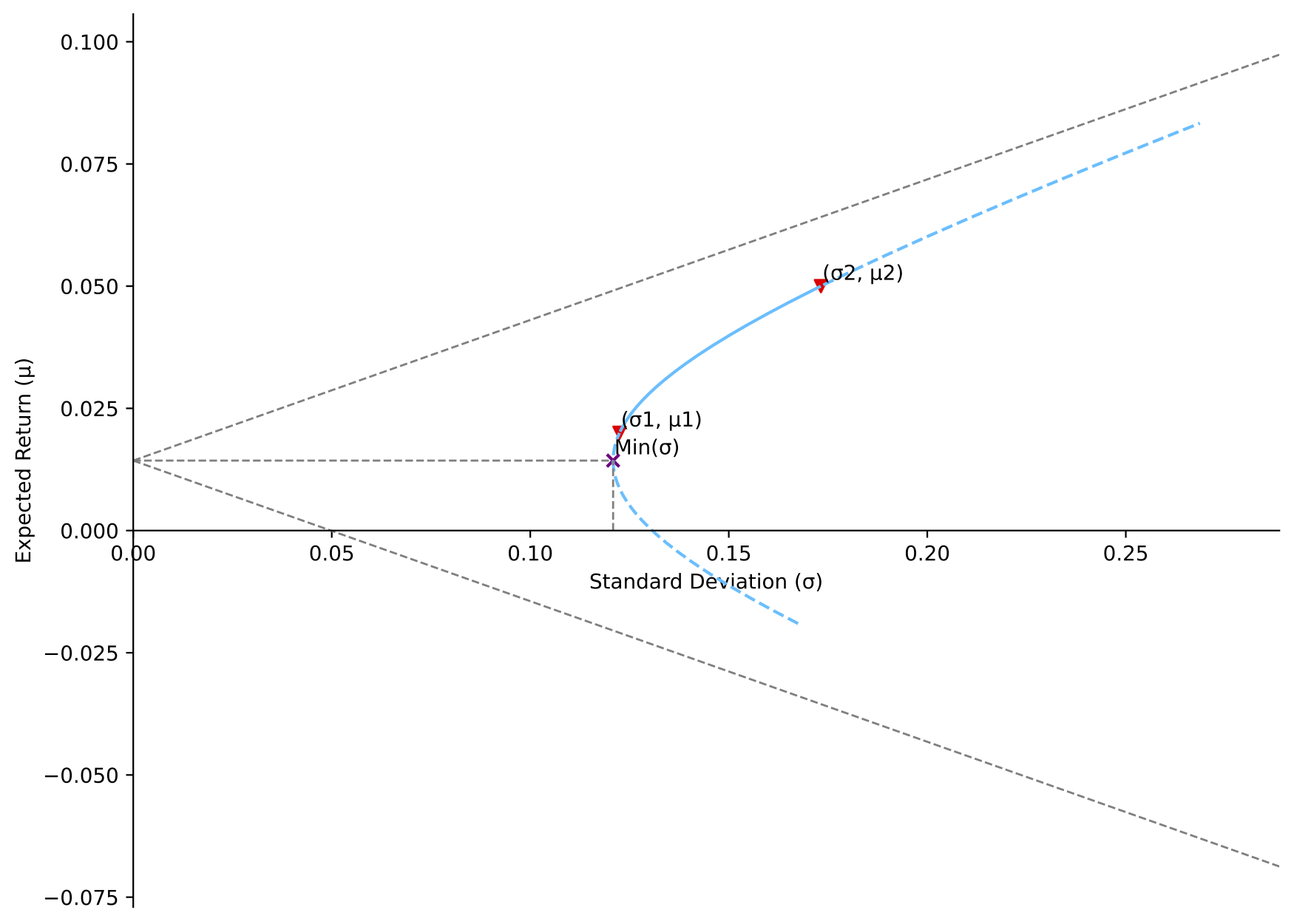
mu1 = 0.02
mu2 = 0.05
var1 = 0.015
var2 = 0.03
corr12 = [1, random.uniform(np.sqrt(var1)/np.sqrt(var2), 1), np.sqrt(var1)/np.sqrt(var2),
random.uniform(-1, np.sqrt(var1)/np.sqrt(var2)), -1]
if var1>0 and var2>0 and var1 != var2:
for situation in map(lambda x: two_asset_plot(mu1, mu2, var1, var2, x), corr12):
situation
else:
print("Error: reset variance")
[Situation 1]: correlation equals 1
MVP strategy (weight): long asset 1 (341.42%), and short asset 2 (-241.42%)
Return of MVP: -0.0524
Minimum variance: 0.0
Covariance: 0.0212
[Situation 2]: correlation between STD1/STD2 (0.7071) and 1
MVP strategy (weight): long asset 1 (118.95%), and short asset 2 (-18.95%)
Return of MVP: 0.0143
Minimum variance: 0.0146
Covariance: 0.0171
[Situation 3]: correlation equals STD1/STD2 (0.7071)
MVP strategy (weight): long asset 1 (100.0%), and ignore asset 2 (0.0%)
Return of MVP: 0.02
Minimum variance: 0.015
Covariance: 0.015
[Situation 4]: correlation between -1 and STD1/STD2 (0.7071)
MVP strategy (weight): long asset 1 (59.75%), and long asset 2 (40.25%)
Return of MVP: 0.0321
Minimum variance: 0.0025
Covariance: -0.016
[Situation 5]: correlation equals -1
MVP strategy (weight): long asset 1 (58.58%), and long asset 2 (41.42%)
Return of MVP: 0.0324
Minimum variance: 0.0
Covariance: -0.0212
## Aggregated plot for the five situations

# corr12 = [1, random.uniform(np.sqrt(var1)/np.sqrt(var2), 1), np.sqrt(var1)/np.sqrt(var2),
#           random.uniform(-1, np.sqrt(var1)/np.sqrt(var2)), -1]

two_asset_plot(mu1, mu2, var1, var2, corr12, separate_plot=False)
STD1/STD2 = 0.7071
[Situation 1] MVP: (0.0, -0.0524), covariance = 0.0212;
MVP strategy (weight): long asset 1 (341.42%), and short asset 2 (-241.42%)
[Situation 2] MVP: (0.1209, 0.0143), covariance = 0.0171;
MVP strategy (weight): long asset 1 (118.95%), and short asset 2 (-18.95%)
[Situation 3] MVP: (0.1225, 0.02), covariance = 0.015;
MVP strategy (weight): long asset 1 (100.0%), and ignore asset 2 (0.0%)
[Situation 4] MVP: (0.0504, 0.0321), covariance = -0.016;
MVP strategy (weight): long asset 1 (59.75%), and long asset 2 (40.25%)
[Situation 5] MVP: (0.0, 0.0324), covariance = -0.0212;
MVP strategy (weight): long asset 1 (58.58%), and long asset 2 (41.42%)
If the portfolio is constructed by one risky asset (expected return: $\mu_1$, variance: $\sigma_1 > 0$) and one risk-free asset (expected return: $R$, variance: 0), the variance of the portfolio would be:
\[\begin{equation} \sigma_V = |w_1| \sigma_1 \end{equation}\]# Special situation: when asset 2 is risk free
mu1_rrf = 0.04
mu2_rrf = 0.01
var1_rrf = 0.03
var2_rrf = 0
corr12_rrf = 0
two_asset_plot(mu1_rrf, mu2_rrf, var1_rrf, var2_rrf, corr12_rrf)
[Special situation]: one risky, another risk free
MVP strategy (weight): ignore asset 1 (0.0%), and long asset 2 (100.0%)
Return of MVP: 0.01
Minimum variance: 0.0
Covariance: 0.0
Example with financial data
For convenience, below provides an example using the monthly value-weighted returns of the portfolio sorted on variance decile, from the Fama/French Data Library.
See pandas-datareader for a wider range of data choices using DataReader.
df = pdr.DataReader('Portfolios_Formed_on_VAR', 'famafrench')
df_vwr = df[0].progress_apply(lambda x: x*0.01)

df_vwr.head(10)
| Lo 20 | Qnt 2 | Qnt 3 | Qnt 4 | Hi 20 | Lo 10 | Dec 2 | Dec 3 | Dec 4 | Dec 5 | Dec 6 | Dec 7 | Dec 8 | Dec 9 | Hi 10 | |
|---|---|---|---|---|---|---|---|---|---|---|---|---|---|---|---|
| Date | |||||||||||||||
| 2017-04 | 0.0169 | 0.0033 | 0.0050 | 0.0087 | -0.0028 | 0.0192 | 0.0135 | 0.0030 | 0.0040 | 0.0074 | 0.0016 | 0.0081 | 0.0097 | 0.0069 | -0.0150 |
| 2017-05 | 0.0241 | -0.0045 | -0.0107 | -0.0037 | -0.0142 | 0.0253 | 0.0214 | -0.0021 | -0.0069 | -0.0198 | -0.0002 | -0.0224 | 0.0183 | -0.0056 | -0.0269 |
| 2017-06 | -0.0047 | 0.0270 | 0.0252 | 0.0226 | 0.0346 | 0.0003 | -0.0109 | 0.0302 | 0.0183 | 0.0259 | 0.0239 | 0.0117 | 0.0344 | 0.0221 | 0.0579 |
| 2017-07 | 0.0203 | 0.0181 | 0.0241 | 0.0095 | 0.0273 | 0.0141 | 0.0276 | 0.0162 | 0.0225 | 0.0235 | 0.0249 | 0.0116 | 0.0074 | 0.0331 | 0.0200 |
| 2017-08 | 0.0079 | 0.0061 | -0.0074 | -0.0185 | -0.0084 | 0.0104 | 0.0049 | 0.0125 | -0.0084 | -0.0093 | -0.0047 | -0.0277 | -0.0083 | -0.0241 | 0.0115 |
| 2017-09 | 0.0217 | 0.0188 | 0.0362 | 0.0526 | 0.0444 | 0.0092 | 0.0374 | 0.0261 | 0.0085 | 0.0328 | 0.0426 | 0.0517 | 0.0536 | 0.0311 | 0.0731 |
| 2017-10 | 0.0304 | 0.0257 | 0.0062 | 0.0214 | -0.0219 | 0.0310 | 0.0293 | 0.0322 | 0.0164 | 0.0017 | 0.0161 | 0.0166 | 0.0270 | -0.0208 | -0.0237 |
| 2017-11 | 0.0340 | 0.0287 | 0.0358 | 0.0313 | 0.0322 | 0.0345 | 0.0335 | 0.0320 | 0.0247 | 0.0584 | 0.0164 | 0.0247 | 0.0356 | 0.0238 | 0.0485 |
| 2017-12 | 0.0120 | 0.0095 | 0.0197 | 0.0002 | 0.0235 | 0.0053 | 0.0193 | 0.0103 | 0.0084 | 0.0205 | 0.0190 | -0.0004 | 0.0016 | 0.0191 | 0.0299 |
| 2018-01 | 0.0483 | 0.0560 | 0.0554 | 0.1001 | 0.0414 | 0.0282 | 0.0691 | 0.0567 | 0.0542 | 0.0633 | 0.0461 | 0.1221 | 0.0515 | 0.0397 | 0.0440 |
def two_asset_series_plot(df, first_col, second_col):
    mu1 = df.mean().loc[first_col]
    mu2 = df.mean().loc[second_col]
    var1 = (df.std().loc[first_col])**2
    var2 = (df.std().loc[second_col])**2
    corr12 = df[first_col].corr(df[second_col], method='pearson', min_periods=None)
    return two_asset_plot(mu1, mu2, var1, var2, corr12)
# choose any two of the portfolios on variance decile

two_asset_series_plot(df_vwr, "Dec 2", "Dec 7")
[Situation 2]: correlation between STD1/STD2 (0.6532) and 1
MVP strategy (weight): long asset 1 (152.11%), and short asset 2 (-52.11%)
Return of MVP: 0.0141
Minimum variance: 0.0018
Covariance: 0.003